Machine Learning Tutorial: Predicting Car Prices with K-Nearest Neighbours (KNN) Regression
Predicting Car Prices with KNN Regression
In this brief tutorial I am going to run through how to build, implement, and cross-validate a simple k-nearest neighbours (KNN) regression model. Simply put, KNN model is a variant of simple linear regression wherein we utilize information about neighbouring data points to predict an unknown outcome. To put a more concrete spin on this, and use the name quite literally, we can think about this in the context of your next door neighbours. If the outcome I wanted to predict was your personal income and didn’t have any other information about you, besides where you live, I might be wise to just ask your next door neighbours. I might decide to run a real life 4-nearest neighbours test. The two houses to the right of yours have a household incomes of $65,000 and $90,000 respectively, and the two to the left $100,000 and $72,000. In the simplest possible fashion I would then just assume you make somewhere in the ballpark of what your neighbours make, take an average, and predict that you have a household income of $81,750.
This is an extremely basic explanation of how KNN algorithms work. But how do we decide who someone’s “neighbours” are when we aren’t talking about literal neighbours? That is, how do we know what other observations are similar to our target? Enter: distance metrics. The most common distance metric in for knn regression problems is Euclidian distance. This isn’t meant to be an extremely math heavy tutorial, so suffice it to say that in running a knn model, for each and every observation in a data set where we want to predict an outcome we grab their k-nearest neighbours, as defined by a metric such as Euclidean distance, from the training set, look at their values for the main dependent variable, and predict the new value based on the neighbours (e.g., as an average in a regression problem, or a “majority vote” in a classification problem).
KNN regression can be used for both classification (i.e., predicting a binary outcome) and regression (i.e., predicting a continuous outcome). The procedure for implementation is largely the same and in this post I’m going to focus on regression. Specifically, the question at hand is: can we predict how much a used car is going to sell for? For this question I am going to utilize a data set from the machine learning repository at The University of California, Irvine. First up is to just take a brief look at what is actually in the dataset.
Brief Exploratory Analysis and Cleaning
These data contain a ton of information on a lot of different cars. For the purposes of this tutorial, I’m just going to pull out a set of relevant columns and work with those.
import pandas as pd

# Need to specify the headers for this dataset
cols = ["symboling", "normalized_losses", "make", "fuel_type", "aspiration",
       "num_doors", "body_style", "drive_wheels", "engine_location",
       "wheel_base", "length", "width", "height", "curb_weight", "engine_type",
       "num_cylinders", "engine_size", "fuel_system", "bore", "stroke",
       "compression_ratio", "horsepower", "peak_rpm", "city_mpg", "highway_mpg",
       "price"]
cars = pd.read_csv("imports-85.data", names=cols)
cars.dtypes
symboling              int64
normalized_losses     object
make                  object
fuel_type             object
aspiration            object
num_doors             object
body_style            object
drive_wheels          object
engine_location       object
wheel_base           float64
length               float64
width                float64
height               float64
curb_weight            int64
engine_type           object
num_cylinders         object
engine_size            int64
fuel_system           object
bore                  object
stroke                object
compression_ratio    float64
horsepower            object
peak_rpm              object
city_mpg               int64
highway_mpg            int64
price                 object
dtype: object
So, as you can see we’ve got 25 columns that might be informative in predicting a car’s sale price, ranging from both highway and city miles per gallon to the number of doors a car has. Let’s take a quick look at the first few rows of the data just so we can get a sense of how it actually looks.
cars.head()
| symboling | normalized_losses | make | fuel_type | ... | horsepower | peak_rpm | city_mpg | highway_mpg | price | |
|---|---|---|---|---|---|---|---|---|---|---|
| 0 | 3 | ? | alfa-romero | gas | ... | 111 | 5000 | 21 | 27 | 13495 |
| 1 | 3 | ? | alfa-romero | gas | ... | 111 | 5000 | 21 | 27 | 16500 |
| 2 | 1 | ? | alfa-romero | gas | ... | 154 | 5000 | 19 | 26 | 16500 |
| 3 | 2 | 164 | audi | gas | ... | 102 | 5500 | 24 | 30 | 13950 |
| 4 | 2 | 164 | audi | gas | ... | 115 | 5500 | 18 | 22 | 17450 |
5 rows × 26 columns
To keep things simple and focus just on numeric columns without much feature engineering for now, it seems like we can use wheelbase, length, width, height, engine size, compression ratio, and city/highway mpr to predict price. Some of these predictors probably offer more information that others (miles per gallon is probably more informative of a car’s sale price than curb weight).
We’re probably going to want to use some of the other variables that aren’t numeric - they are likely also meaningful. So, right now we’ll deal with counting and seeing where our missing values are, as well as turning relevant columns numeric so we can actually use them. You will have noticed above that there were some questionmarks in the data - we just need to turn those into missing values. So I do this in the code below, then I select sex non-numeric columns that might be meaningful (normalized_losses, bore, stroke, horsepower, peak_rpm, and price) and turn them numeric. These ones are easy as they are actually numbers, they just are currently stored as objects.
import numpy as np

cars = cars.replace('?', np.nan)

# Now lets make things numeric
num_vars = ['normalized_losses', "bore", "stroke", "horsepower", "peak_rpm",
            "price"]

for i in num_vars:
    cars[i] = cars[i].astype('float64')

cars.head()
| symboling | normalized_losses | make | fuel_type | ... | horsepower | peak_rpm | city_mpg | highway_mpg | price | |
|---|---|---|---|---|---|---|---|---|---|---|
| 0 | 3 | NaN | alfa-romero | gas | ... | 111.0 | 5000.0 | 21 | 27 | 13495.0 |
| 1 | 3 | NaN | alfa-romero | gas | ... | 111.0 | 5000.0 | 21 | 27 | 16500.0 |
| 2 | 1 | NaN | alfa-romero | gas | ... | 154.0 | 5000.0 | 19 | 26 | 16500.0 |
| 3 | 2 | 164.0 | audi | gas | ... | 102.0 | 5500.0 | 24 | 30 | 13950.0 |
| 4 | 2 | 164.0 | audi | gas | ... | 115.0 | 5500.0 | 18 | 22 | 17450.0 |
5 rows × 26 columns
Everything looks good now - how many missing values do we have in the normalized losses column?
print("normalized losses: ", cars['normalized_losses'].isnull().sum())
normalized losses: 41
There are 41 missing values in the normalized_losses column. Given there are only 205 rows, thats a decent chunk missing. I’m not sure this column is the most useful, so we’ll just not use this column in our analyses at all. Let’s take a look at our other numeric columns and see what the missing values are like. The below chunk just calculates the sum of missing values for each variable and displays that sum.
cars.isnull().sum()
symboling             0
normalized_losses    41
make                  0
fuel_type             0
aspiration            0
num_doors             2
body_style            0
drive_wheels          0
engine_location       0
wheel_base            0
length                0
width                 0
height                0
curb_weight           0
engine_type           0
num_cylinders         0
engine_size           0
fuel_system           0
bore                  4
stroke                4
compression_ratio     0
horsepower            2
peak_rpm              2
city_mpg              0
highway_mpg           0
price                 4
dtype: int64
So it looks like most of our columns are pretty good, with only a couple missing values here and there. The most crucial one here is price, our dependent variable; there are four cars that don’t have prices. Given that the number of missing rows is, at most, about 2%, I’m just going to listwise delete any row that has a missing variable in any of these. I don’t like mean imputation as it is purely making up data.
I’ll start with the price column because its the most important and I suspect the rows that are missing price are the same rows missing the other data as well. Here I just drop any rows that are missing price data:
cars = cars.dropna(subset = ['price'])
Now lets check the missing values again, just to be sure it worked correctly:
cars.isnull().sum()
symboling             0
normalized_losses    37
make                  0
fuel_type             0
aspiration            0
num_doors             2
body_style            0
drive_wheels          0
engine_location       0
wheel_base            0
length                0
width                 0
height                0
curb_weight           0
engine_type           0
num_cylinders         0
engine_size           0
fuel_system           0
bore                  4
stroke                4
compression_ratio     0
horsepower            2
peak_rpm              2
city_mpg              0
highway_mpg           0
price                 0
dtype: int64
Now, I’ll do the same to listwise delete the other numeric columns.
cars = cars.dropna(subset = ['bore', 'stroke', 'horsepower', 'peak_rpm'])
Now, we should have no missing data and be ready to go! The next step is to convert all the numeric columns into standardized z-scores. This is especially important if your variables are on drastically different scales. For instance here, horsepower is generally way up over 100 and miles per gallon is never more than about 45. So what I’ll do below is trim the dataset down just to the numeric columns, and then convert each of those columns into a z-score. Then, I save this into a new dataset called “normalized.” This is generally good practice because that way we retain our original dataset in case we need to go back to it.
cols = ['wheel_base', 'length', 'width', 'height',
        'curb_weight', 'engine_size', 'bore', 'stroke', 'horsepower',
        'peak_rpm', 'city_mpg', 'highway_mpg', 'price']
cars = cars[cols]

normalized_cars = (cars - cars.mean()) / (cars.std())
Modeling
Alright, onward into some modeling! We’ve got a nice clean data set full of numeric columns. The first thing I’m going to do is create a couple of univariate (i.e., just one predictor) models, just to see how informative certain predictors are. Now, in more traditionally academic regression contexts this would be akin to just running some linear regressions with individual predictors. For example, we might see how well highway miles per gallon “predicts” sale price on it’s own. Of course, in the academic context, when we say predict what we actually mean is “variance explained” - we’re really finding out how much of the variance in sale price can be explained just by looking at highway miles per gallon.
In the machine learning context, we are actually more concerned with prediction. That is, if we build a KNN model, where we were only identifying neighbours based on how similar they were in highway miles per gallon, could we accurately predict price? There are myriad different ways we could judge accuracy, but here I’m going to use Root Mean Squared Error (RMSE). RMSE is one of the most common error metrics for regression based machine learning. Again, this is not meant to be a math-heavy tutorial so I won’t go into it deeply here but it quantifies how far off our predictions were from the actual values.
So, to start running some very basic univariate KNN models I imported two pieces of the sklearn package below, one for training a KNN model (KNeighborsRegressor) and one for calculating the mean squared error (mean_squared_error), from which we will derive the RMSE. Now, we need to do a couple things to build these models. Specifically, we need to choose the predictor we want to test, choose the dependent variable, and split our data into training and test sets so we reduce the risk of overfitting.
To accomplish this, I define a function that takes in three arguments: (1) our training column(s), (2), our target column, and (3) the dataset to use. Using this information, the function first instatiates an instance of a k-nearest neighbours regression (stored as “knn”) and sets a set so our results are reproducible. Next, the function shuffles the data into a random order, splits the data in half, designates the top half as the training data, and the bottom half as the test data.
Then, we get down to the nitty gritty. The function fits the knn object on the specified training and test columns of the training data, uses that model to make predictions on the test data, and then calculates the RMSE (e.g., the difference between the predictions our model made for each car in the test set’s price and the actual prices).
As we move through, we’ll complicate this function bit by bit, adding extra stuff to it.
# Writing a simple function that trains and tests univariate models
# This function takes in three arguments: the predictor, the outcome, & the data
from sklearn.neighbors import KNeighborsRegressor
from sklearn.metrics import mean_squared_error

def knn_train_test(train_col, target_col, df):
    knn = KNeighborsRegressor()
    np.random.seed(1)

    # Randomize order of rows in data frame.
    shuffled_index = np.random.permutation(df.index)
    rand_df = df.reindex(shuffled_index)

    # Divide number of rows in half and round.
    last_train_row = int(len(rand_df) / 2)

    # Select the first half and set as training set.
    # Select the second half and set as test set.
    train_df = rand_df.iloc[0:last_train_row]
    test_df = rand_df.iloc[last_train_row:]

    # Fit a KNN model using default k value.
    knn.fit(train_df[[train_col]], train_df[target_col])

    # Make predictions using model.
    predicted_labels = knn.predict(test_df[[train_col]])

    # Calculate and return RMSE.
    mse = mean_squared_error(test_df[target_col], predicted_labels)
    rmse = np.sqrt(mse)
    return rmse
Now that we’ve got this function defined, let’s use it! If you recall, I said I was going to just test some basic univariate models. So, I’m going to run our new function five times, getting the RMSE of five different predictors. I just chose four that I thought would be relatively meaningful in predicting price (city and highway miles per gallon, engine size, and horsepower) and one to serve as a logic check (width) - why would width predict the price of a car, unless larger vehicles are more expensive. In any case, my intuition suggests that width should be the word predictor of price.
# Lets test a couple of predictors
print('city mpg: ', knn_train_test('city_mpg', 'price', normalized_cars))
print('width: ', knn_train_test('width', 'price', normalized_cars))
print('highway mpg: ', knn_train_test('highway_mpg', 'price', normalized_cars))
print('engine size: ', knn_train_test('engine_size', 'price', normalized_cars))
print('horsepower: ', knn_train_test('horsepower', 'price', normalized_cars))
city mpg:  0.598975486019
width:  0.671608148246
highway mpg:  0.537913994132
engine size:  0.536691465842
horsepower:  0.571585852136
As I suspected, width is by quite a large margin the worst predictor of a car’s price. Of the couple predictors that I threw in there to test, the best most informative for determining a vehicles price seems to be it’s highway. So, if we wanted to be as accurate as possible while only using on predictor, we would want to use fuel economy on the highway.
“Hyperparamaterization”
If you recall, in KNN regression, we can set k to be whatever we want: 3, 5, 7, 100, 1000. Common values of k range from 3 to 10 - does tweaking our k value, and grabbing more or less neighbours to make our price guess, make the model fit better? As a test of this question, I’m going to modify the above function to take another argument: a k value. Then, I’ll test each of the five predictors above (plus some more) each with five different values of k (1, 3, 5, 7, and 9). This will effectively run our regression 25 times; city mpg with 1 neighbour, city mpg with 2 neighbours, and so on.
The way I’ve done this is to insert a list of k-values into the middle of the function, and set up an empty dictionary to store all our RMSEs. Then, I nested the code from previously that fits the model, generates our predictions, and calculates the RSME into a for loop that does this for each value of k. Lastly, it appends the RMSE to the dictionary and returns it.
Lastly, I specified a list of all the columns I want to build univariate models for, use a for loop to run the function on each of those columns, and append the results to another dictionary called “k_rmse_results.” Printing this dictionary gives us the name of the predictor, the specified k, and then the RMSE.
def knn_train_test_new(train_col, target_col, df):
    np.random.seed(1)

    # Randomize order of rows in data frame.
    shuffled_index = np.random.permutation(df.index)
    rand_df = df.reindex(shuffled_index)

    # Divide number of rows in half and round.
    last_train_row = int(len(rand_df) / 2)

    # Select the first half and set as training set.
    # Select the second half and set as test set.
    train_df = rand_df.iloc[0:last_train_row]
    test_df = rand_df.iloc[last_train_row:]

    k_values = [1,3,5,7,9]
    k_rmses = {}

    for k in k_values:
        # Fit model using k nearest neighbors.
        knn = KNeighborsRegressor(n_neighbors=k)
        knn.fit(train_df[[train_col]], train_df[target_col])

        # Make predictions using model.
        predicted_labels = knn.predict(test_df[[train_col]])

        # Calculate and return RMSE.
        mse = mean_squared_error(test_df[target_col], predicted_labels)
        rmse = np.sqrt(mse)

        k_rmses[k] = rmse
    return k_rmses

k_rmse_results = {}

# For each column from above, train a model, return RMSE value
# and add to the dictionary `rmse_results`.
variables = ['wheel_base', 'length', 'width', 'height',
        'curb_weight', 'engine_size', 'bore', 'stroke', 'horsepower',
        'peak_rpm', 'city_mpg', 'highway_mpg']

for var in variables:
    rmse_val = knn_train_test_new(var, 'price', normalized_cars)
    k_rmse_results[var] = rmse_val

k_rmse_results
{'bore': {1: 1.2142304178718561,
  3: 0.86766581048215152,
  5: 0.89458788943880752,
  7: 0.94676716177240661,
  9: 0.95385344053196963},
 'city_mpg': {1: 0.69529747854104784,
  3: 0.59031417913396289,
  5: 0.59897548601904338,
  7: 0.59715938629269016,
  9: 0.57728649652220132},
 'curb_weight': {1: 0.8365387787670262,
  3: 0.64395375801733934,
  5: 0.57031290606074236,
  7: 0.51644149986604171,
  9: 0.51839468763038343},
 'engine_size': {1: 0.55456842477058543,
  3: 0.54125650939355474,
  5: 0.53669146584152094,
  7: 0.51899873944760311,
  9: 0.50362821678292591},
 'height': {1: 1.1521894508998922,
  3: 1.0168354498989998,
  5: 0.94018342361170537,
  7: 0.98192402693779424,
  9: 0.94562106614391528},
 'highway_mpg': {1: 0.69402405950428248,
  3: 0.57416390399142236,
  5: 0.53791399413219376,
  7: 0.53495996840130122,
  9: 0.54899088943686292},
 'horsepower': {1: 0.54931712010379319,
  3: 0.58337889657418729,
  5: 0.57158585213578872,
  7: 0.59314672824644243,
  9: 0.59002690698940097},
 'length': {1: 0.65713817747103875,
  3: 0.63950652453727652,
  5: 0.64700844560860649,
  7: 0.66892394999830362,
  9: 0.6572441270128111},
 'peak_rpm': {1: 0.85899385207057188,
  3: 0.88634665981443039,
  5: 0.90984280257609562,
  7: 0.90757986581712302,
  9: 0.90022237747155309},
 'stroke': {1: 0.91796375714948086,
  3: 0.88113492952413897,
  5: 0.89586641314603555,
  7: 0.94574853212680499,
  9: 0.92121730389055356},
 'wheel_base': {1: 0.70984063675235898,
  3: 0.70981264790591259,
  5: 0.70662378566203043,
  7: 0.71073380297018984,
  9: 0.72499494497288963},
 'width': {1: 0.77543242861316763,
  3: 0.68812005931548847,
  5: 0.67160814824580428,
  7: 0.5826291501627695,
  9: 0.56790774193128279}}
Generally speaking, just eyeballing within each predictor, going up to k = 9 worked the best for some of the models, but not for others. The error actually went up as we increased k for some. With a k of 9, the best univariate predictor seems to be engine size, with predictions only off by about half a standard deviation. So thats the best so far, but it’s still not great. When trying to predict an outcome, univariate models aren’t going to be extremely informative. Outcomes are complex, so let’s build a model that reflects that and takes in more than one column.
What I’ve done to accomplish this is modified the above function to take multiple columns and then train and test some models using the the best two, then three, four, and five columns from above. By eyeballing at the 5-nearest neighbours level, the columns that predict the best in isolation are engine size, highway mpg, curb_weight, horsepower, and city mpg.
def knn_train_test_mult(train_cols, target_col, df):
    np.random.seed(1)

    # Randomize order of rows in data frame.
    shuffled_index = np.random.permutation(df.index)
    rand_df = df.reindex(shuffled_index)

    # Divide number of rows in half and round.
    last_train_row = int(len(rand_df) / 2)

    # Select the first half and set as training set.
    # Select the second half and set as test set.
    train_df = rand_df.iloc[0:last_train_row]
    test_df = rand_df.iloc[last_train_row:]

    k_values = [5]
    k_rmses = {}

    for k in k_values:
        # Fit model using k nearest neighbors.
        knn = KNeighborsRegressor(n_neighbors=k)
        knn.fit(train_df[train_cols], train_df[target_col])

        # Make predictions using model.
        predicted_labels = knn.predict(test_df[train_cols])

        # Calculate and return RMSE.
        mse = mean_squared_error(test_df[target_col], predicted_labels)
        rmse = np.sqrt(mse)

        k_rmses[k] = rmse
    return k_rmses

train_cols_2 = ['engine_size', 'highway_mpg']
train_cols_3 = ['engine_size', 'highway_mpg', 'curb_weight']
train_cols_4 = ['engine_size', 'highway_mpg', 'curb_weight',
               'horsepower']
train_cols_5 = ['engine_size', 'highway_mpg', 'curb_weight',
               'horsepower', 'city_mpg']

k_rmse_results = {}

rmse_val = knn_train_test_mult(train_cols_2, 'price', normalized_cars)
k_rmse_results["two best features"] = rmse_val
rmse_val = knn_train_test_mult(train_cols_3, 'price', normalized_cars)
k_rmse_results["three best features"] = rmse_val
rmse_val = knn_train_test_mult(train_cols_4, 'price', normalized_cars)
k_rmse_results["four best features"] = rmse_val
rmse_val = knn_train_test_mult(train_cols_5, 'price', normalized_cars)
k_rmse_results["five best features"] = rmse_val

k_rmse_results
{'five best features': {5: 0.49634970383078636},
 'four best features': {5: 0.48157162981314988},
 'three best features': {5: 0.50707231602531166},
 'two best features': {5: 0.43695579560820619}}
So, what we have here is four new models that combine the best features we identified above. For example, the two best features model is using engine size and highway mpg to predict sale price with k set to 5. The three best predictors model is using engine size, highway mpg, and curb weight. Interestingly, adding more predictors does not increase the performance of the model at all - in fact, it makes it worse. This is not at all surprising because we started with the two best predictors, and just tacked on worse and worse predictors. So simply adding more doesn’t do anything good for us, it just adds muddier predictors to the model.
The best performing model here to predict the price of a car is simply it’s engine size and highway miles per gallon. Let’s combine the two tests we’ve done so far and go a little overboard with it. Let’s test are four multivariate models at all ks ranging from 1 to 25.
def knn_train_test_mult(train_cols, target_col, df):
    np.random.seed(1)

    # Randomize order of rows in data frame.
    shuffled_index = np.random.permutation(df.index)
    rand_df = df.reindex(shuffled_index)

    # Divide number of rows in half and round.
    last_train_row = int(len(rand_df) / 2)

    # Select the first half and set as training set.
    # Select the second half and set as test set.
    train_df = rand_df.iloc[0:last_train_row]
    test_df = rand_df.iloc[last_train_row:]

    k_values = list(range(1,25))
    k_rmses = {}

    for k in k_values:
        # Fit model using k nearest neighbors.
        knn = KNeighborsRegressor(n_neighbors=k)
        knn.fit(train_df[train_cols], train_df[target_col])

        # Make predictions using model.
        predicted_labels = knn.predict(test_df[train_cols])

        # Calculate and return RMSE.
        mse = mean_squared_error(test_df[target_col], predicted_labels)
        rmse = np.sqrt(mse)

        k_rmses[k] = rmse
    return k_rmses

k_rmse_results_2 = {}

rmse_val = knn_train_test_mult(train_cols_2, 'price', normalized_cars)
k_rmse_results_2["two best features"] = rmse_val
rmse_val = knn_train_test_mult(train_cols_3, 'price', normalized_cars)
k_rmse_results_2["three best features"] = rmse_val
rmse_val = knn_train_test_mult(train_cols_4, 'price', normalized_cars)
k_rmse_results_2["four best features"] = rmse_val
rmse_val = knn_train_test_mult(train_cols_5, 'price', normalized_cars)
k_rmse_results_2["five best features"] = rmse_val

k_rmse_results_2
{'five best features': {1: 0.48370851070283638,
  2: 0.45709593736092696,
  3: 0.45932846135166017,
  4: 0.47702516372024495,
  5: 0.49634970383078636,
  6: 0.51326367838750764,
  7: 0.49909158266517145,
  8: 0.49234720868686166,
  9: 0.49925986215124729,
  10: 0.50320132862625788,
  11: 0.49352187011331128,
  12: 0.50969596379759741,
  13: 0.51666729281793589,
  14: 0.52430330537451841,
  15: 0.52831175797337293,
  16: 0.53372729477563852,
  17: 0.53629514907736431,
  18: 0.53771760713738892,
  19: 0.54366780131360726,
  20: 0.55390626006954025,
  21: 0.56186625263562961,
  22: 0.56399228907515964,
  23: 0.56686293421110434,
  24: 0.56749133395228601},
 'four best features': {1: 0.46011695087263338,
  2: 0.47254209382853879,
  3: 0.4957675847479055,
  4: 0.47457606714743178,
  5: 0.48157162981314988,
  6: 0.4988487989184765,
  7: 0.51321993316267744,
  8: 0.51485477394479984,
  9: 0.51767653423898286,
  10: 0.5323478616627898,
  11: 0.51621784291210482,
  12: 0.51180481420952084,
  13: 0.52093660357028182,
  14: 0.5264585716201885,
  15: 0.53375627848681184,
  16: 0.53867876043121632,
  17: 0.539751445854185,
  18: 0.54052905274747964,
  19: 0.54394381259000146,
  20: 0.55263828123323866,
  21: 0.55895871633176053,
  22: 0.56273074037859749,
  23: 0.55965116497813094,
  24: 0.56079209060485291},
 'three best features': {1: 0.53304672541629627,
  2: 0.47236953984714419,
  3: 0.48544239785342919,
  4: 0.46468465687861726,
  5: 0.50707231602531166,
  6: 0.50672338800144279,
  7: 0.52042141176821866,
  8: 0.51959755832321974,
  9: 0.51531096459267978,
  10: 0.52080169867439063,
  11: 0.52322240088596494,
  12: 0.52075280982124794,
  13: 0.51183217030638006,
  14: 0.51868070682253542,
  15: 0.52774088364145721,
  16: 0.53035523273810814,
  17: 0.53183552745587126,
  18: 0.53451532836203997,
  19: 0.54155167597224763,
  20: 0.54551779898598018,
  21: 0.54674295619522062,
  22: 0.54707824469373634,
  23: 0.54985793303062935,
  24: 0.55512440029648535},
 'two best features': {1: 0.4962211708123152,
  2: 0.42439666654800412,
  3: 0.37244955551446796,
  4: 0.38221587546513652,
  5: 0.43695579560820619,
  6: 0.49363489340281513,
  7: 0.50823941279743867,
  8: 0.51418965195989808,
  9: 0.52616341995960625,
  10: 0.53013621032483371,
  11: 0.53671709358748898,
  12: 0.53444184258976579,
  13: 0.51587142155192167,
  14: 0.51205713655316698,
  15: 0.5119686970820041,
  16: 0.51750488428455055,
  17: 0.52218955380387977,
  18: 0.53175784405886029,
  19: 0.54377416147308744,
  20: 0.54302569583633942,
  21: 0.54968364588915308,
  22: 0.5508362135961884,
  23: 0.55132842211110611,
  24: 0.55665088230669157}}
As you can probably tell, it’s hard to make sense of this. For our different models with 2, 3, 4, and 5 predictors, what is the most accurate value of k? The best way to explore this might be just to plot it out! So, I’ll take the big dictionary that’s printed above and plot it out with RMSE on the y axis, k on the x axis, and then each colored line is a different model.
import matplotlib.pyplot as plt
% matplotlib inline

for k,v in k_rmse_results_2.items():
    x = list(v.keys())
    y = list(v.values())

    plt.plot(x,y)
    plt.xlabel('k value')
    plt.ylabel('RMSE')

plt.show()
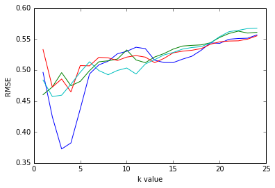
The pattern you can discern just looking at the numbers becomes clear here when looking at the graph. The best models for any given set of predictors is right around a k of 3-5. Once we start adding more than that, the performance of the model gets worse.
Conclusion
So, we’ve learned a lot about how to run a KNN regression using python, how to tweak paramaters like the number of predictors in a model and the number of neighbors we use, and how to evaluate those models.
From this, we learned in our simple set of predictions that the most accurate model is using just the two best predictors, engine size and highway miles per gallon, with k set somewhere in the 3-5 range.
I hope you found this tutorial helpful, and I encourage you to give it a shot for yourself using this dataset, or any other, from UCI’s rich machine learning repository!